
TL;DR
- The entire pipeline — ~1,000 lines of Python, 60+ API calls, seven visualizations, a statistical report, and a fraud-similarity model — was built in Claude Code sessions.
- The pipeline failed three times before it worked. DMEPOS data had zero NPI overlap with LEIE. The default CMS API returned 2013 data. Florida alone produced only 28 matches. Each failure required a pivot — from DMEPOS to Part B, from one state to ten, and eventually to all states.
- A data bug inflated the cohort 3× and survived initial review. Excluded providers appeared in multiple state/year datasets because the pipeline loaded full billing files. The fix was one filter — but finding it required understanding the join logic across five functions.
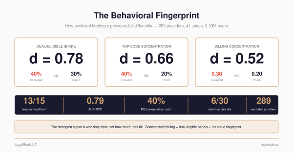
- **Excluded providers show a detectable behavioral fingerprint.** 13 of 15 features significant after Bonferroni correction, but the resulting screen is false-positive dominated. Full results in the companion post.
- Twelve search methods failed before one worked. justice.gov is JavaScript-rendered. Google blocks scripts. Bing serves CAPTCHAs. The Tavily API via MCP was the only method that returned results — 17 DOJ prosecution matches from 43 providers searched.
- **A logistic regression ranks every provider by similarity to excluded providers — AUC 0.79, not a calibrated fraud probability.** The sklearn implementation is in this post; the full results and manual public-record check are in the companion post.
- You can reproduce this analysis yourself. The full
backtest.py, the data sources, and the commands are in this post.pip install pandas scipy matplotlib requests pyarrow scikit-learnandpython backtest.py.
Update, June 24, 2026: This walkthrough was tightened to match the corrected results post: §1128(b)(7) is now described as fraud, kickbacks, and other prohibited activities rather than excessive services; the model score is framed as a similarity score rather than a calibrated probability; and the high-scoring-peer check is described as a manual public-record check, not proof of model lift.
The previous post reported what the backtest found — 13 significant features, a fraud-similarity model at AUC 0.79, and a manual public-record check of high-scoring peers. This post is the build log: how the pipeline was constructed, the three times it failed, and the engineering decisions that shaped the final design.
The Spec#
The starting point was a paragraph:
Durable medical equipment — wheelchairs, oxygen tanks, prosthetics — is one of Medicare’s most fraud-prone billing categories, and the OIG regularly excludes DME suppliers. CMS publishes annual DMEPOS billing summaries keyed on NPI. Cross-reference the two: do excluded suppliers show detectable billing anomalies in the year before exclusion?
Two public federal datasets make this possible. The OIG LEIE (List of Excluded Individuals and Entities) is the federal government’s exclusion list — every provider barred from billing Medicare, with their NPI, exclusion date, and reason. CMS DMEPOS files are the billing side — annual summaries of what every Medicare equipment supplier billed, how many beneficiaries they served, and how much they charged. Match the two and you can see what an excluded supplier’s billing looked like before exclusion. Both datasets appeared in earlier posts in this series. The usual toolkit for this kind of pipeline is pandas, scipy, matplotlib, requests, and a weekend. Claude Code compressed the timeline — one session that ran overnight instead of a weekend.
First Attempt: DME Suppliers#
First target: DMEPOS (durable medical equipment) suppliers — a category the OIG has flagged as particularly fraud-prone. This depended on the LEIE being able to identify which excluded providers were DME suppliers. The LEIE’s GENERAL and SPECIALTY fields might not be granular enough to isolate them, so the pipeline’s first step was a verification check — each NPI’s taxonomy code against the NPPES registry before pulling billing data.
The taxonomy check killed the approach:
[3/5] NPPES taxonomy verification ...
  Checking 47 NPIs against NPPES ...
  DME suppliers (taxonomy 332B00000X): 0
Zero. The LEIE’s excluded providers in Florida are overwhelmingly individual healthcare workers — doctors, nurses, therapists. The specialty fields don’t reliably distinguish DME suppliers from other provider types. Without a clean way to identify DME suppliers in the exclusion list, there was no cohort to build.
One more check confirmed the structural problem went deeper than labeling:
# Quick check: how many LEIE NPIs appear in DMEPOS data?
leie_npis = set(cohort_df["NPI"])
dmepos_npis = set(dmepos_df["Rfrng_NPI"].astype(str))
overlap = leie_npis & dmepos_npis
print(f"Overlap: {len(overlap)}")
# Overlap: 0
Zero overlap between the two datasets entirely. DMEPOS billing data is 99.5% organizational NPIs (Type 2) — companies, not people. LEIE exclusions are individual providers (Type 1). Even if the specialty labeling were perfect, the entity types don’t align across these datasets.
Lesson: The OIG excludes people. CMS DMEPOS data tracks organizations. The join between the two doesn’t exist in these datasets — though CMS PECOS enrollment files publish ownership relationships that could bridge the gap. That’s a more complex pipeline for another day. The faster path: pivot to data that already tracks individual providers.
Second Attempt: Part B Individual Providers#
The Type 1/Type 2 mismatch pointed directly to the fix: CMS Part B Provider Utilization data tracks individual physician billing — the same entity type as LEIE. Rebuilt the pipeline against Part B instead of DMEPOS. New problem:
  Fetching CMS Part B data...
  Provider rows: 1,023,847
  Checking NPI overlap...
  Matched: 0 of 248
Zero again. The default CMS API endpoint was returning the oldest available data (2013). Providers excluded in 2022–2023 weren’t billing Medicare in 2013 — or if they were, under different NPIs.
CMS publishes Part B data as year-specific datasets, each with its own UUID. The default endpoint returns the oldest vintage, not the most recent. The fix: pull the correct UUIDs from the data.cms.gov catalog API:
CMS_PROVIDER_UUIDS = {
    2017: "44ea2789-993f-4d55-ac44-ed7f160b58fa",
    2018: "900850df-c9a9-47ce-a9e0-d0ceae5a811f",
    2019: "6a53afe5-1cbc-4b33-9dc8-926ee532dc66",
    2020: "29d799aa-c660-44fe-a51a-72c4b3e661ac",
    2021: "44e0a489-666c-4ea4-a1a2-360b6cdc19db",
    2022: "21555c17-ec1b-4e74-b2c6-925c6cbb3147",
}
With year-specific data, the pipeline matched excluded NPIs to the year before their exclusion — the billing year that shows what the provider looked like while still practicing.
Florida, 2020 billing data, providers excluded 2022–2023:
  Matched: 28 of 248
  Statistical comparison:
    * dual_share          d=+0.72  p=0.0001
    * top_hcpcs_share     d=+0.33  p=0.0028
      services_per_bene   d=+0.12  p=0.0842
Signal exists — dual-eligible share and billing concentration both significantly different. But 28 providers is thin for statistical power. Only two features survived Bonferroni correction.
Expansion to Ten States#
The statistics need at least 100 to be credible, which meant expanding beyond Florida. The LEIE data showed clear volume clusters — Florida, Texas, California, New York, and a handful of other states account for the bulk of exclusions. Next step: scale the pipeline to the top ten states by LEIE volume, with exclusion dates from 2020–2023 and six years of billing data to search.
Back-of-envelope math: ~745 excluded NPIs across ten states, ~11% match rate based on the Florida run, projected yield around 130–200. Enough to get past the power threshold.
The expanded pipeline required significant restructuring. The key design change: for each excluded provider, find the best available billing year — the most recent CMS data before their exclusion date. A provider excluded in March 2022 checks 2021 first, then 2020, then 2019, walking backward until a match is found.
def find_best_billing_year(cohort_df):
    for state, npis in npis_by_state.items():
        for year in sorted(CMS_PROVIDER_UUIDS.keys(), reverse=True):
            remaining = npis - found_in_state
            eligible = {n for n in remaining
                        if excl_year_map.get(n, 9999) > year}
            provider_df = download_cms_state_year(state, year, "provider")
            matched = eligible & set(provider_df["Rndrng_NPI"])
            for npi in matched:
                results.append({"NPI": npi,
                                "billing_year": year,
                                "billing_state": state})
This triggered 60+ API calls — one per state per year, paginated at 5,000 rows per page, with exponential backoff on failures. Each state-year combo cached to parquet after first download. Total data: 1.7 GB across 3.4 million provider rows and 28.9 million service-level rows.
[3/5] Finding best billing year per provider ...
  Searching CA (207 NPIs) ... found 63, missing 144
  Searching FL (248 NPIs) ... found 67, missing 181
  Searching GA (45 NPIs) ... found 14, missing 31
  Searching IL (36 NPIs) ... found 17, missing 19
  Searching MI (61 NPIs) ... found 29, missing 32
  Searching NJ (35 NPIs) ... found 10, missing 25
  Searching NY (150 NPIs) ... found 42, missing 108
  Searching OH (211 NPIs) ... found 30, missing 181
  Searching PA (95 NPIs) ... found 23, missing 72
  Searching TX (149 NPIs) ... found 51, missing 98
  Total matched: 346 of 1237
  By billing year: {2017: 51, 2018: 74, 2019: 85,
                    2020: 54, 2021: 51, 2022: 31}
346 matched providers. The 72% miss rate is itself a finding. Some of those missing providers likely stopped billing Medicare before their exclusion date — the pipeline only covers six years of billing data, and some exclusions lag practice by years. Others may never have billed Medicare at all; the OIG excludes providers for license revocations, felonies, and drug convictions, and some of those providers may have only treated private-pay or Medicaid patients. Those are guesses that would need to be tested against the actual exclusion-type breakdown.
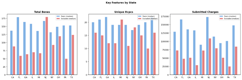
The signal wasn’t uniform across states. Florida and California had the deepest cohorts (67 and 63 matched providers), while New Jersey contributed only 10. More importantly, the magnitude of the gap between excluded and peer providers varied — some states showed excluded providers billing far fewer unique codes than peers, while others showed the gap mostly in beneficiary counts or submitted charges.
The Data Duplication Bug#
The first run of the expanded pipeline reported:
Excluded: 1056, Peers: 2,862,7511,056 excluded rows from 346 unique NPIs. Something was wrong.
The cause: the pipeline loads all provider data for each state-year combination needed by any excluded NPI. If Florida has excluded NPIs with billing years 2019, 2020, and 2021, it loads the full Florida provider file for all three years. An excluded NPI assigned to 2020 also appeared in the 2019 and 2021 datasets — and the code marked them “excluded” in all rows.
The fix was one filter:
# Only include each excluded NPI in their assigned billing year/state
npi_year = dict(zip(matched["NPI"],
                     matched["billing_year"].astype(int)))
npi_state = dict(zip(matched["NPI"],
                      matched["billing_state"]))
excl_rows = provider_df_filtered[
    provider_df_filtered["Rndrng_NPI"].isin(excluded_npis)
    & provider_df_filtered.apply(
        lambda r: r["_year"] == npi_year.get(r["Rndrng_NPI"])
        and r["_state"] == npi_state.get(r["Rndrng_NPI"]),
        axis=1,
    )
]
After the fix: 346 excluded rows, 346 unique NPIs. The signal actually got stronger — the duplicated rows had been diluting the effect sizes with out-of-window billing data.
Lesson: Data duplication bugs in multi-table joins are silent. The statistical tests still ran. The p-values still looked significant. The effect sizes were just smaller than they should have been, which looks like a weak signal, not a bug. Without checking unique NPI counts against row counts, this would have shipped.
All States and Fraud-Specific Exclusions#
The next iteration addressed two weaknesses: geographic scope and cohort precision.
Geographic expansion. Restricting to ten states was an artifact of the original design — pick the highest-volume states, get enough providers for statistical power, move on. But it left 40 states unexamined and raised the question of whether the fingerprint was a regional pattern or a national one. Removing the state filter and querying CMS Part B data for every state in the LEIE yielded 41 states with at least one matched provider. The pipeline’s download logic already handled arbitrary state lists, so the code change was minimal — the API calls were not. Every new state required its own set of year-specific downloads.
Exclusion type filtering. The original cohort included all Section 1128 exclusion types — including §1128(b)(4) (license revocations) and §1128(a)(4) (controlled substance convictions), which have nothing to do with billing fraud. A provider excluded for a DUI-related license revocation shouldn’t dilute a billing fraud fingerprint. The refined cohort restricts to three fraud-specific provisions: §1128(a)(1) (program-related convictions), §1128(a)(3) (felony convictions related to health care fraud), and §1128(b)(7) (fraud, kickbacks, and other prohibited activities). This dropped the matched count from 346 to 289 — a smaller but cleaner cohort.
The full statistical results from this final cohort — including the complete feature table, effect sizes, and significance tests — are in the results post.
The Working Pipeline#
The final pipeline (backtest.py) runs end-to-end with python backtest.py. It:
- Downloads and caches the LEIE (83,256 records, ~16 MB CSV) from oig.hhs.gov
- Builds the excluded cohort — filters to selected fraud-specific exclusion types (§1128(a)(1), (a)(3), (b)(7)), 2018–2023 exclusions, valid NPIs, all states
- Finds best billing year — for each NPI, walks backward through CMS Part B datasets (2022 → 2017) until it finds a match → 289 matched across 41 states
- Downloads billing data — provider-level and service-level CMS Part B data for every state-year combination needed, cached to parquet
- Builds peer groups — same state, same specialty, same year, ≥11 beneficiaries → 3,393,561 peers
- Computes 15 features — volume metrics, intensity ratios, concentration indices, demographic indicators
- Runs statistical comparison — Mann-Whitney U, Welch’s t-test, Cohen’s d, Bonferroni correction
- Trains fraud-similarity model — logistic regression ranking every provider by similarity to excluded providers (AUC 0.79)
- Generates seven visualizations — box plots, radar chart, scatter plot, heatmap, state-level comparison, risk distribution, feature importance
- Matches DOJ prosecutions — cross-references cohort against curated
doj_matches.json(17 confirmed federal cases) - Writes
report.md— cohort summary, full statistical table, model results, prosecution matches, high-scoring-peer public-record checks, key findings, caveats
Total runtime on cached data: ~2 minutes. First run (all downloads): ~45 minutes depending on CMS API response times.
The Results#
The full statistical breakdown — 13 of 15 features significant after Bonferroni correction, three with large effect sizes — is in the results post. The practice-size confound analysis and caveats are there too.
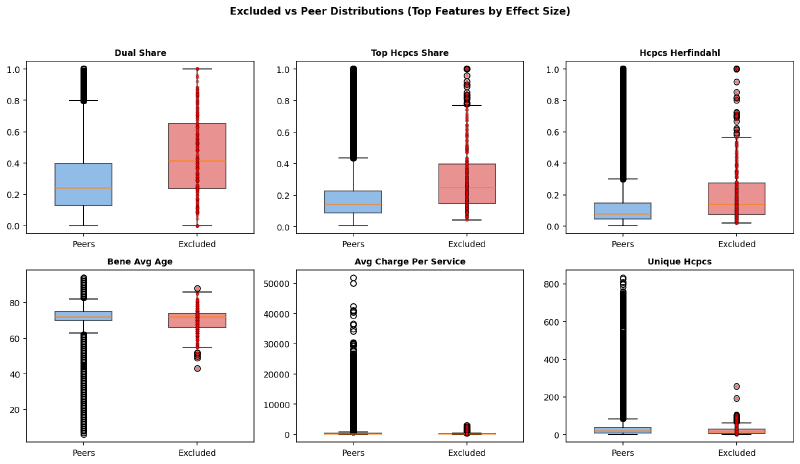
What the walkthrough adds is the visualizations that show how the data separates — views that didn’t make it into the results post because they illustrate the analysis process rather than the findings.
The top six features by effect size show clear shifts between excluded and peer populations — not just in the median, but in the spread:
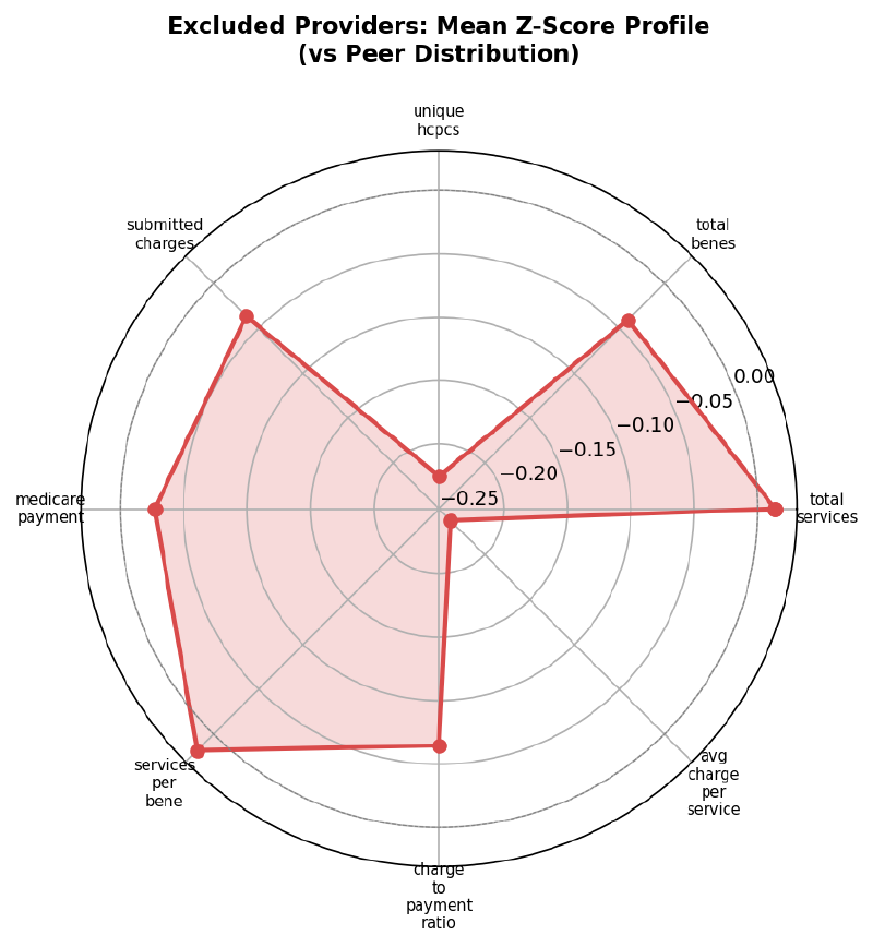
Each axis of the radar chart is a feature’s mean Z-score for excluded providers relative to peers. The shape reveals the composite pattern — higher on services_per_bene and submitted_charges, lower on unique_hcpcs, avg_charge_per_service, and medicare_payment:
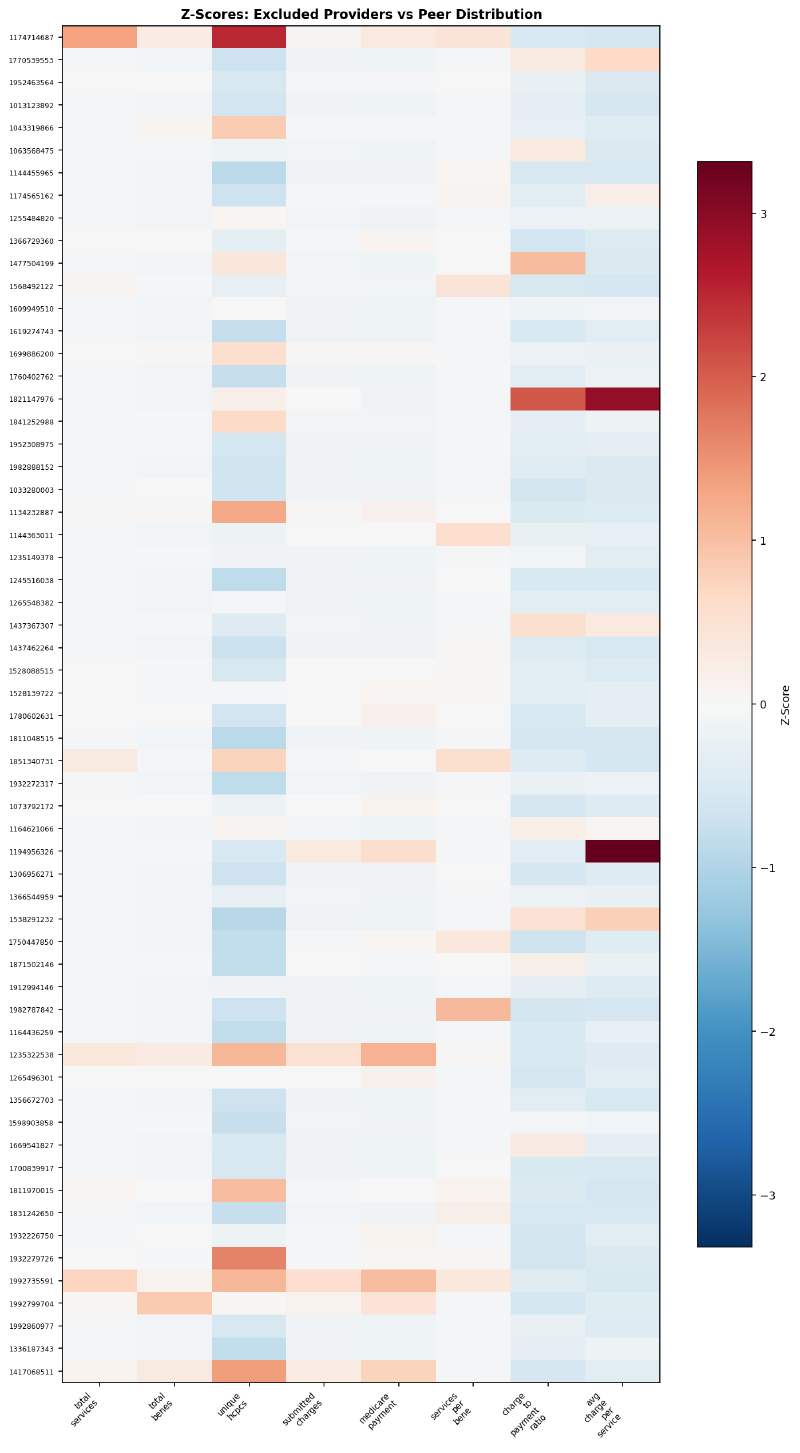
Individual providers don’t all match the aggregate pattern. The heatmap shows Z-scores for a sample of excluded providers — each row is one NPI, each column is a feature. Some providers are extreme on one dimension but normal on others:
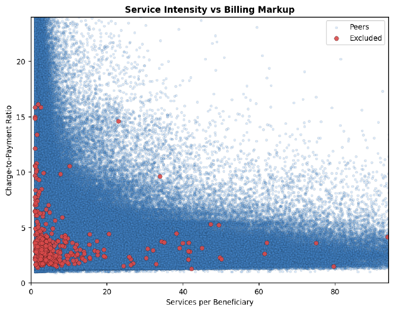
Services per beneficiary against charge-to-payment ratio — a proxy for billing intensity vs. markup. Excluded providers (red) cluster in the low-services, moderate-markup region:
Prosecution Matching#
Do these excluded providers correspond to real federal fraud cases with named defendants and prison sentences?
The goal was straightforward — search each excluded provider’s name plus state against DOJ press releases on justice.gov. The execution was not.
The Search API Graveyard#
Twelve methods failed before one worked:
justice.gov/search— JavaScript-rendered, returns empty HTML to scriptssearch.justice.gov— same problem, React single-page appsearch.usa.govAPI — requires an API key- Google via
requests— blocked - Google via
googlesearch-python— empty results - Bing via
requests— CAPTCHA - DuckDuckGo HTML/lite — empty results
duckduckgo-searchpackage — broken/renamed- Playwright headless on Google — “unusual traffic” block
- Playwright headless on DuckDuckGo — empty results
- DOJ JSON API / RSS feeds — all 404
- Direct
curlto DuckDuckGo — empty
The only method that worked: the Tavily search API via
MCP, querying "Provider Name" medicare fraud State restricted to justice.gov. Searched in batches of five to stay within rate limits.
Results#
43 excluded providers searched, 17 confirmed federal prosecution matches — a 40% hit rate against DOJ press releases. The full prosecution table, state-by-state match rates, and the analysis of why the 40% is a floor for this specific press-release search are in the results post.
Pipeline Integration#
The prosecution matching was added as step [6/6] in backtest.py:
def load_doj_matches():
    """Load curated DOJ prosecution matches from data/doj_matches.json"""
    with open("data/doj_matches.json") as f:
        return json.load(f)

def match_prosecutions(cohort_df, doj_matches):
    """Cross-reference excluded cohort with DOJ press releases"""
    matched = cohort_df[cohort_df["NPI"].isin(
        [m["npi"] for m in doj_matches]
    )]
    return matched
The doj_matches.json and peer_validations.json files were force-committed to git, bypassing the data/ gitignore. Unlike the cached CMS downloads, these are curated research data that don’t regenerate from an API call — doj_matches.json has 17 prosecution entries with NPIs, DOJ URLs, and sentences; peer_validations.json has the 6 public-record enforcement hits from the manual public-record check step.
The report now includes a linked provider table and state-level match rates alongside the statistical results.
The Risk Model#
Logistic regression with balanced class weights — standard handling for extreme imbalance (289 excluded vs. 3.39 million peers). StandardScaler on features, 5-fold stratified cross-validation. The implementation emits a score between 0 and 1 for every provider, but because of the class weighting and extreme imbalance, that score is a similarity ranking — not a calibrated probability of fraud.
from sklearn.linear_model import LogisticRegression
from sklearn.preprocessing import StandardScaler
from sklearn.model_selection import StratifiedKFold, cross_val_predict

scaler = StandardScaler()
X_scaled = scaler.fit_transform(X)
model = LogisticRegression(class_weight="balanced", max_iter=1000)
risk_scores = cross_val_predict(model, X_scaled, y,
                                cv=StratifiedKFold(5, shuffle=True),
                                method="predict_proba")[:, 1]
The model produced a cross-validated AUC-ROC of 0.792. At a 0.9 threshold, it still flags 22,410 active peers — 0.66% of the 3.39 million peer set — so the output is a false-positive-dominated triage screen, not a fraud list. Feature importance, score distributions, and the full interpretation are in the results post.
The Manual Public-Record Check#
Searching public records for the 30 highest-scoring peer providers turned up 6 with confirmed enforcement actions — including a $7M Medicare fraud conviction — none of which were in the training labels. This shows that the model surfaces some providers with independent enforcement histories outside the LEIE labels. It does not prove lift over chance, because the search did not include a matched low-scoring control group. The full manual-check results and the structural NPI gap they revealed are in the results post.
What Claude Code Did and Didn’t Do#
Claude Code wrote every line of Python — the download logic, the caching layer, the statistical tests, the visualizations. What it didn’t do: choose the research question, select the datasets, decide when to pivot, or catch the duplication bug. Each pivot in this post — DMEPOS to Part B, single-state to ten, fixing the join logic — required understanding the data well enough to diagnose what went wrong and decide what to try next.
This is the division of labor described in Claude for Legal Work: the analyst directs, the AI builds.
Reproduce It#
The full pipeline is at legalrealist/backtest-poc — the repo contains backtest.py, a README with setup instructions, the curated doj_matches.json prosecution data, and the generated report and visualizations for reference. It runs on a reasonably provisioned machine with Python 3.10+, several GB of disk space, and an internet connection. No API keys required.
git clone https://github.com/legalrealist/backtest-poc.git
cd backtest-poc
pip install pandas scipy matplotlib requests pyarrow scikit-learn
python backtest.py
First run downloads ~4 GB of CMS data from three public federal APIs, cached to data/ as parquet files for subsequent runs. Outputs: report.md and seven PNGs in figures/.
The Data Access Code#
Three data sources, no API keys. The LEIE is a single CSV. CMS Part B data is trickier — each billing year is a separate dataset with its own UUID, and the default API endpoint returns the oldest vintage, not the most recent.
Dataset UUIDs. CMS publishes Part B data as year-specific datasets on data.cms.gov. These UUIDs are not discoverable from the API itself — they come from the catalog. Provider-level data (one row per NPI per state per year) and service-level data (one row per NPI per HCPCS code) use different dataset IDs:
CMS_PROVIDER_UUIDS = {
    2017: "44ea2789-993f-4d55-ac44-ed7f160b58fa",
    2018: "900850df-c9a9-47ce-a9e0-d0ceae5a811f",
    2019: "6a53afe5-1cbc-4b33-9dc8-926ee532dc66",
    2020: "29d799aa-c660-44fe-a51a-72c4b3e661ac",
    2021: "44e0a489-666c-4ea4-a1a2-360b6cdc19db",
    2022: "21555c17-ec1b-4e74-b2c6-925c6cbb3147",
}

CMS_SERVICE_UUIDS = {
    2017: "85bf3c9c-2244-490d-ad7d-c34e4c28f8ea",
    2018: "fb6d9fe8-38c1-4d24-83d4-0b7b291000b2",
    2019: "867b8ac7-ccb7-4cc9-873d-b24340d89e32",
    2020: "c957b49e-1323-49e7-8678-c09da387551d",
    2021: "31dc2c47-f297-4948-bfb4-075e1bec3a02",
    2022: "e650987d-01b7-4f09-b75e-b0b075afbf98",
}
Paginated fetch. The CMS API returns at most 5,000 rows per request. A single state-year can have 50,000+ providers, requiring 10+ pages. The pipeline paginates with exponential backoff on failures:
def fetch_cms_paginated(dataset_id, params, label):
    base_url = f"https://data.cms.gov/data-api/v1/dataset/{dataset_id}/data"
    page_size = 5000
    offset = 0
    all_rows = []
    while True:
        p = {**params, "size": page_size, "offset": offset}
        resp = requests.get(base_url, params=p, timeout=120)
        resp.raise_for_status()
        rows = resp.json()
        if not rows:
            break
        all_rows.extend(rows)
        offset += page_size
    return pd.DataFrame(all_rows)
State-year caching. Each state-year download is cached to parquet. The pipeline makes 60+ API calls on first run — one per state per year per data type — but subsequent runs read from disk in seconds:
def download_cms_state_year(state, year, kind):
    uuids = CMS_PROVIDER_UUIDS if kind == "provider" else CMS_SERVICE_UUIDS
    cache = Path(f"data/cms_{kind}_{state}_{year}.parquet")
    if cache.exists():
        return pd.read_parquet(cache)

    df = fetch_cms_paginated(
        uuids[year],
        {"filter[Rndrng_Prvdr_State_Abrvtn]": state},
        f"{kind} {state} {year}",
    )
    if not df.empty:
        df.to_parquet(cache)
    return df
LEIE download. The exclusion list is a single CSV. The full pipeline refreshes the local copy when stale; the simplified read step looks like this:
LEIE_URL = "https://oig.hhs.gov/exclusions/downloadables/UPDATED.csv"
leie_df = pd.read_csv("data/UPDATED.csv", dtype={"NPI": str})
The data sources:
- LEIE: oig.hhs.gov/exclusions/downloadables/UPDATED.csv — the OIG exclusion list (83K+ records, ~16 MB)
- CMS Part B Provider: data.cms.gov API — year-specific dataset UUIDs above
- CMS Part B Service-level: Same API, service-level dataset UUIDs above
The raw CMS billing data (~4 GB of parquet files) is too large to include in the repo — the pipeline downloads and caches it on first run. The LEIE updates regularly as providers are added and removed, so a stale snapshot would produce different results than a fresh download; the pipeline refreshes the local copy before analysis. The curated research data — doj_matches.json (prosecution matches) and peer_validations.json (high-scoring-peer public-record checks) — is included in the repo since it doesn’t regenerate from an API call.
If you’d rather skip the 45-minute first-run download and work with the cached data directly, reach out — happy to provide it.
Every result in the analysis above can be reproduced from these sources. The complete pipeline — including cohort building, feature computation, statistical tests, the fraud-similarity model, and report generation — is in backtest.py in the repo.
Further Reading#
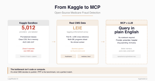
- From Kaggle to MCP: Open-Source Medicare Fraud Detection. The data landscape, open-source repos, and five data access proposals.
- Show Your Work: The Open-Source PPP Fraud Analysis. The PPP pipeline this backtest is modeled after.
- DOJ Health Care Fraud Unit. Federal prosecution press releases and Strike Force operations.
- Claude Code. The AI coding assistant used to build the pipeline.
- CMS Part B Provider Utilization Data. The billing data API.
- OIG LEIE Exclusion Database. The exclusion list.
- OIG Exclusion Authorities. Statutory basis for exclusion types.
- NPPES NPI Registry. Provider identity verification.
- data.cms.gov. The CMS open data portal.
- Herfindahl-Hirschman Index. The concentration metric.
- Mann-Whitney U Test. The non-parametric group comparison test.
- Bonferroni Correction. Multiple comparison adjustment.
This post is part of the Data Analytics and Fraud series on LegalRealist AI. It is intended for informational and educational purposes only and does not constitute legal advice. The analysis described here uses publicly available CMS data and OIG exclusion records; no patient-level or claim-level data was accessed. Statistical findings describe population-level differences and do not constitute evidence of fraud for any individual provider. The pipeline code and methodology are provided for educational and research purposes. AI capabilities, data availability, and enforcement practices described here reflect publicly available information as of the publication date and are subject to change. Laws governing healthcare fraud, data privacy, and qui tam litigation vary by jurisdiction.